Exomoon Transits

In Spring of 2022, I joined an exoplanet research group led by Professor Eric Agol at the University of Washington. PhD candidate at the time, Tyler Gordon, was who I primarily worked with and from whom I received guidance. Let me first start by defining what an exomoon is for those not familiar: A moon that orbits a planet that orbits a star other than our Sun. They have never been detected, although candidates have arisen from time-to-time.

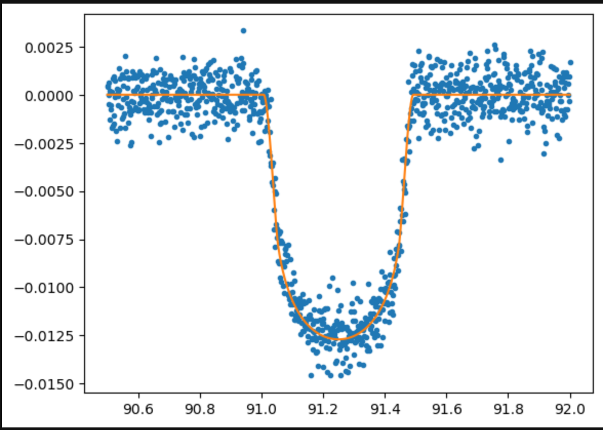
Now, what's a transit? When we say that an exomoon transits a star, we mean that the exoplanet-exomoon system crosses in front of the host star, blocking light from reaching us. If we measure flux (the amount of light per unit area) before, during, and after the transit, we get what is called a light curve, shown to the right. The shape of the resulting light curves depends on the orbits and radii of the transitting bodies. Therefore, hypothetically, we can determine the orbits and radii given the light curve.

Tyler created gefera, a Python package that computes two models: The dynamical model which is used to compute the positions of two bodies at a given time or array of times, and the photometric model which computes the observed flux given the positions of the bodies. The goal of my project was to calculate the information matrix for the 18 parameters that define a transit model.

First, I found that I had to reparameterize the model because the original parameters were too correlated. The original set of parameters and the new set can be found on the right. The conversion between the two can be done with fairly simple orbital mechanics. In order to calculate the information matrix, the derivatives of the light curve with respect to each parameter are needed. This was the part of the project that consumed much of my time. At first glance, it seemed like a simple chain rule problem, but unfortunately that was not the case. It ended up being a system of 18 equations that required manipulation to get the derivatives I wanted. To test the analytical expressions, I compared them to their respective finite differences.

After confirming that the expressions were correct, I sought out to calculate the information matrix. I started simple, though. I only considered the case of the exoplanet and no exomoon. This allowed me to break up the process into two distinct parts so any errors that arose were more traceable. After testing the exoplanet case, I found that there were a couple parameters that were causing problems, so I omitted them from future calculations. This was by no means a hasty decision as much thought went into how to proceed. I decided that getting a working information matrix with some parameters and then going back to make it work with all parameters was the best use of my time.

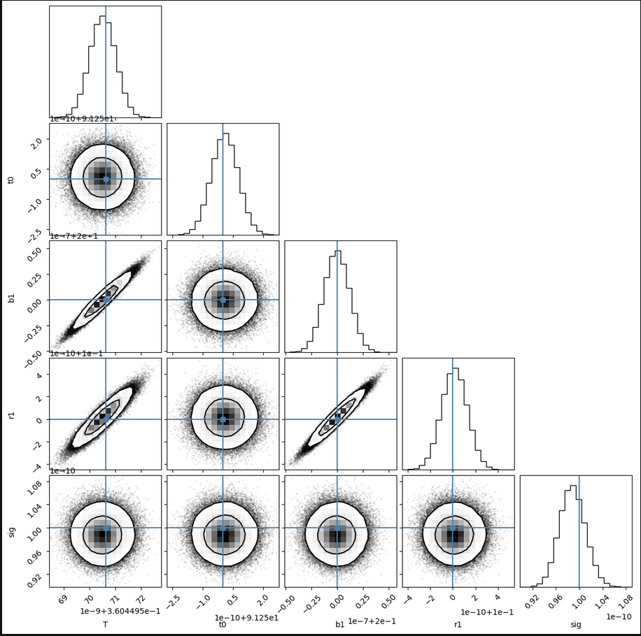
After getting an information matrix that looked reasonable, I shifted my focus to using machine learning to verify that it was right. The method of choice was Markov Chain Monte Carlo (MCMC) because I had experience with using it for similar purposes. Treating its results as the ground truth, I used it to check if my information matrix was correct. A corner plot showing the values of the parameters and the uncertainties as calculated by MCMC is shown at the right. Suffice it say, the uncertainties calculated by my information matrix did not align with the machine learning results.

This is about where I lost momentum as my temporary position as a Research Aide at UW ended and other projects began to take up my time. This project is not abandoned, but rather on hold. I look forward to sharing more as I progress.

Lastly, though not associated with this project, I wrote a short paper for my Exoplanets course about exomoon detection methods. If you are interested in learning more, feel free to download the paper below.

Imaging Globular Cluster M3

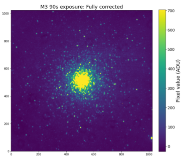
As part of an observational astronomy at the University of Washington, my final project involved remotely connecting to the Apache Point Observatory and taking images of Messier 3, a globular cluster. I worked in a group with three of my classmates and we connected to the telescope together and took turns controlling it and taking pictures. We first had to take calibration images so that we could later correct the pictures of the cluster for any instrumental noise. We then took pictures of M3 at various different exposure times. Shorter exposure times such as 5 seconds were used to better differentiate between the stars towards the center of the cluster, and longer exposure times such as 90 seconds revealed dimmer stars further from the center.

After taking images, I sought out to estimate the age of the cluster by making a color-magnitude diagram and identifying the turn-off point. I communicated my findings in a final paper that you can download below if you have further interest in this experience.

Modelling the Universe

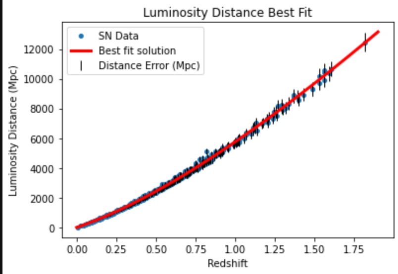
As part of a Cosmology course at the University of Washington, my final project involved using machine learning to determine the composition of a hypothetical universe. I was given data of the distance to supernovae and their redshifts. Redshift refers to the doppler effect in space. As an object in space moves away from us, the wavelength of the light emitted from the object is lengthened. This causes the object to look slightly more red, and the faster the object is moving away from us, the redder it appears.

Using the Python libraries, astropy and emcee, and the popular machine learning method, Markov Chain Monte Carlo (MCMC), I found the values of Ω_m, Ω_Λ, and H₀ that described the cosmology that best fit the supernovae data. Ω_m quantifies the density of non-relativistic matter in the universe. Ω_Λ does the same but for dark energy. H₀ is the Hubble constant, or the rate at which the universe is expanding.

I recommend downloading the html file below to get a better understanding of this project. Looking at the outputs should give you an idea of what values and uncertainties I found. This project served as a simple application of machine learning to astronomy.

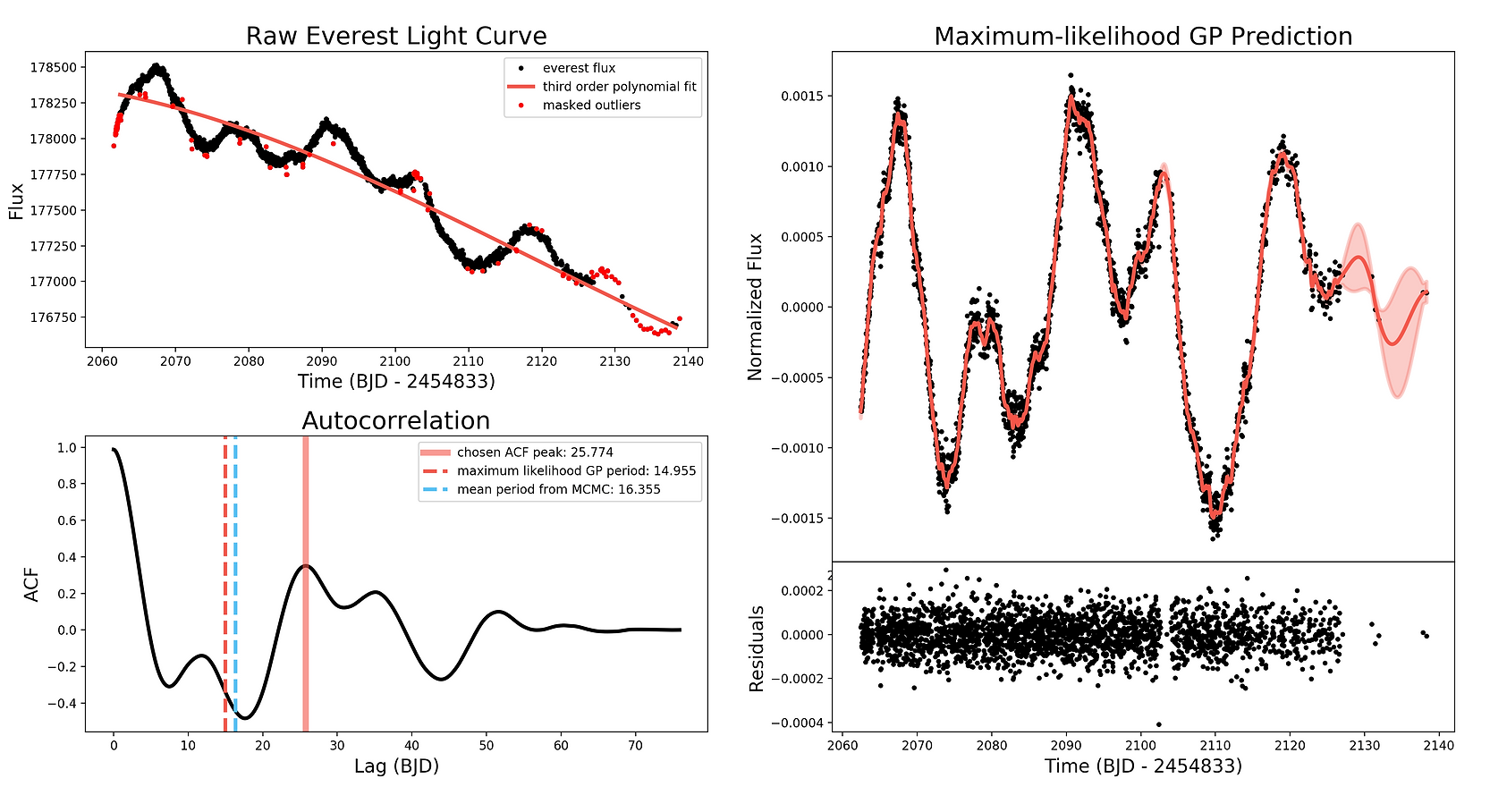
Identifying Stellar Rotation

In my first quarter at the University of Washington, I took a class intended for those planning on majoring in astronomy. This class first covered the basics of python with astronomy applications, and then research with graduate students. One fellow student and I were paired with Tyler Gordon (mentioned in the Exomoon Transits section) and were to help as much as we could with his research. Our goal as assistants was to determine which data points indicated a light curve resembled stellar rotation. To accomplish this goal, we first manually sorted and determined by-eye which light curves from the Kepler K2 mission sample were generated from stellar rotators. We then used python to explore the relationship between different data points and the classification of stellar rotator. For example, we were particularly interested in whether an agreement in period determined by MCMC and Gaussian Processing was indicative of stellar rotation. We evaluated the effectiveness of a particular filter by using an receiver operating characteristic (ROC) curve which shows the false positive and true positive rates of a binary classifier. We presented our findings in a 10 minute presentation to the University of Washington Astronomy Department.

Analyzing Advanced Hockey Statistics

As both a lifetime hockey player and enjoyer of statistics, I am fascinated by hockey statistics and how they can tell interesting stories of players' careers. As a passion project, I learned R to explore the stats behind a Boston Bruins legend, Patrice Bergeron. This project did not start with an ultimate goal in mind, but rather it served as an opportunity to pose interesting questions as I went along. Every time I found an answer, I immediately thought of ten more questions I could explore with R.

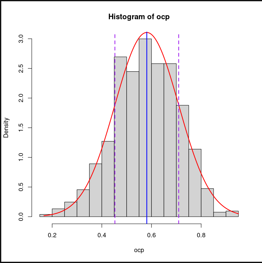
I first started by identifying stats that were regarded by the hockey community to be the best descriptors of success: Corsi percentage and Fenwick percentage. Corsi percentage is defined as the percentage of all shots (including those that miss the net or get blocked) that occur for one's team while the player is on the ice, while Fenwick percentage is the same except for it does not include blocked shots. I plotted the distribution of Bergeron's Corsi and Fenwick percentages and performed simple non-linear regression to fit a Gaussian to them. The distribution was clearly normal, as seen on the right.

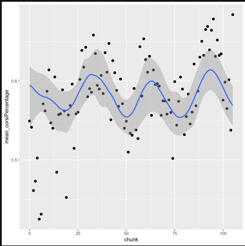
I then was curious how a time series of each of those statistics looked, so I took chunks of 10 games, took the average of each stat, and then plotted sequentially. Upon first plotting these series, I thought that they looked sinusoidal. I then fit simple sine curves to them, fitting only three parameters: the amplitude, frequency, and phase shift. The fits were not even close, so I got a bit more specific. I fit increased the number of parameters to five and used the expression \(A Sin(Bx) + C + D Cos(Ex)\). After some trial and error with different bayesian inference methods, I settled on using the brms library and used its non-linear regression function, brm. The model and its uncertainty is seen on the right. A "chunk" is 10 games.

All in all, this project has served as a way for me to learn more about statistics and data science. This is an ongoing project as I generate more questions I wish to answer. With every question comes a plethora of googling to better understand statistical inference. The current question I am working towards answering is whether other players also experience clear peaks and valleys throughout their careers. To answer this, I must fit a similar model as I did for Bergeron and determine goodness of fit. I look forward to continuing to work on this and I think the results will tell an interesting story.